Matplotlibのサーフェスプロット

公開日 2023-08-16

この記事では、Matplotlibでサーフェスプロットを出力する方法を解説します。サーフェスプロットでは、複数のデータ点に囲まれた面を描画します。

サーフェスプロットの基本

plt.subplots()のsubplot_kwオプションに{'projection': '3d'}という辞書形式データを与えることで、3次元のプロットになります。サーフェスプロットとするには、さらにax.plot_surface()メソッドを使います。

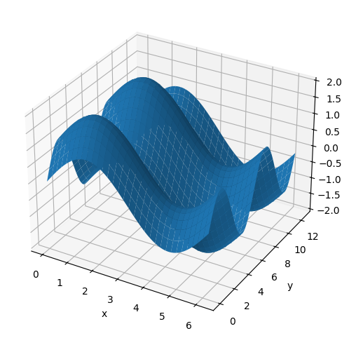
ax.plot_surface()メソッドにはデータ点のx, y, z座標を与えます。以下に例を示します。

import matplotlib.pyplot as plt
import numpy as np

x = np.arange(0, 2*np.pi, 0.1)
y = np.arange(0, 4*np.pi, 0.1)
X, Y = np.meshgrid(x, y)
Z = np.sin(X) + np.sin(Y)

fig, ax = plt.subplots(figsize=(6, 6), subplot_kw={'projection': '3d'})
ax.plot_surface(X, Y, Z)
ax.set_xlabel("x")
ax.set_ylabel("y")
ax.set_zlabel("z")
plt.show()

なお、変数X, Y, Zはいずれも同じ大きさの2次元配列となります。

print(X.shape)
print(Y.shape)
print(Z.shape)

(126, 63)
(126, 63)
(126, 63)

ax.plot_surface()メソッドの主なオプションを以下に示します。

引数	型	説明
rcount, ccount	int	行・列方向の最大サンプル数。データ点数がこれより多い場合、ダウンサンプリングされる（デフォルト値：50）
rstride, cstride	int	ダウンサンプリングするときに飛ばすデータ点数
color	str	面の色
alpha	float	面の透明度
edgecolor	str	枠線の色
cmap	str	面のカラーマップ
vmin, vmax	float	カラーマップ範囲の最小値、最大値
shade	bool	シェーディング（陰影）処理の有無（デフォルト：True）

rcountとrstrideは片方のみ指定できます。同様に、ccountとcstrideも片方のみ指定できます。

データのダウンサンプリング

rcount, rstride, ccount, cstrideで描画する頂点の数を変更できます。

rcount=10, ccount=10として、描画点数をx, y軸方向にそれぞれ10点とした例を以下に示します。デフォルト値 (50) よりもメッシュが荒くなっていることが分かります。

fig, ax = plt.subplots(figsize=(6, 6), subplot_kw={'projection': '3d'})
ax.plot_surface(X, Y, Z, rcount=10, ccount=10)
ax.set_xlabel("x")
ax.set_ylabel("y")
ax.set_zlabel("z")
plt.show()

面の色

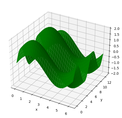
colorオプションで面の色を指定できます。

fig, ax = plt.subplots(figsize=(6, 6), subplot_kw={'projection': '3d'})
ax.plot_surface(X, Y, Z, color="green")
ax.set_xlabel("x")
ax.set_ylabel("y")
ax.set_zlabel("z")
plt.show()

指定可能な色については以下のページを参照下さい。

Matplotlib 色の書式

面の色の透明度

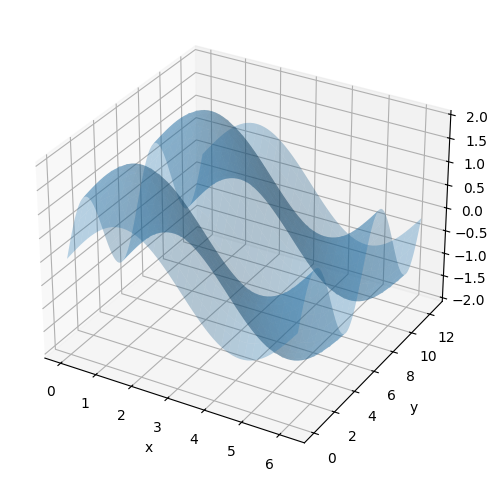
面の色の透明度を指定するには、alphaオプションを使用します。0から1の範囲の値を取り、値が小さいほど透明になります（デフォルトは1）。以下にalpha=0.3とした例を示します。

fig, ax = plt.subplots(figsize=(6, 6), subplot_kw={'projection': '3d'})
ax.plot_surface(X, Y, Z, alpha=0.3)
ax.set_xlabel("x")
ax.set_ylabel("y")
ax.set_zlabel("z")
plt.show()

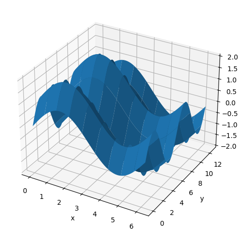
枠線の色

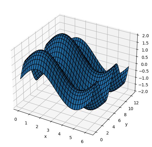
枠線の色をedgecolorオプションで指定できます。

fig, ax = plt.subplots(figsize=(6, 6), subplot_kw={'projection': '3d'})
ax.plot_surface(X, Y, Z, edgecolor="black")
ax.set_xlabel("x")
ax.set_ylabel("y")
ax.set_zlabel("z")
plt.show()

カラーマップ

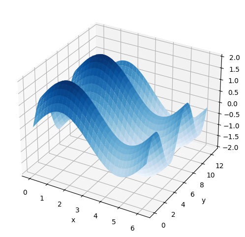
cmapオプションで面のカラーマップを指定できます。z軸の値に応じて面の色が変化します。

fig, ax = plt.subplots(figsize=(6, 6), subplot_kw={'projection': '3d'})
ax.plot_surface(X, Y, Z, cmap="Blues")
ax.set_xlabel("x")
ax.set_ylabel("y")
ax.set_zlabel("z")
plt.show()

指定可能なカラーマップについては以下のページを参照下さい。

Matplotlibのカラーマップ

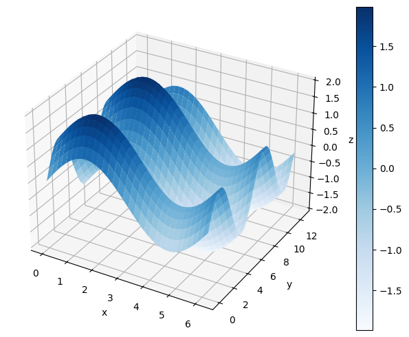
カラーバーを表示する場合、plt.colorbarを使用します。ax.pcolorの戻り値はPolyCollectionというクラスのオブジェクトです。これをplt.colorbarの最初の引数とします。また、axオプションにカラーバーを表示するグラフ（ここではax）を指定します。

fig, ax = plt.subplots(figsize=(8, 5), subplot_kw={'projection': '3d'})
mappable = ax.plot_surface(X, Y, Z, cmap="Blues")
plt.colorbar(mappable, ax=ax)
ax.set_xlabel("x")
ax.set_ylabel("y")
ax.set_zlabel("z")
fig.tight_layout()
plt.show()

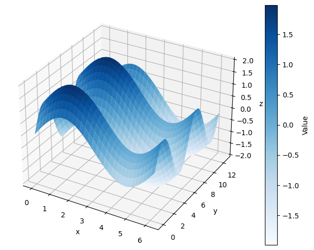
表示するカラーマップの範囲を固定したい場合、最小値と最大値をそれぞれvmin, vmaxで指定します。

カラーバーにラベルを付ける場合、plt.colorbarの戻り値を取得（以下ではcbarとしています）し、この戻り値のset_labelメソッドを使用します。

fig, ax = plt.subplots(figsize=(8, 5), subplot_kw={'projection': '3d'})
mappable = ax.plot_surface(X, Y, Z, cmap="Blues")
cbar = plt.colorbar(mappable, ax=ax)
cbar.set_label('Value')
ax.set_xlabel("x")
ax.set_ylabel("y")
ax.set_zlabel("z")
fig.tight_layout()
plt.show()

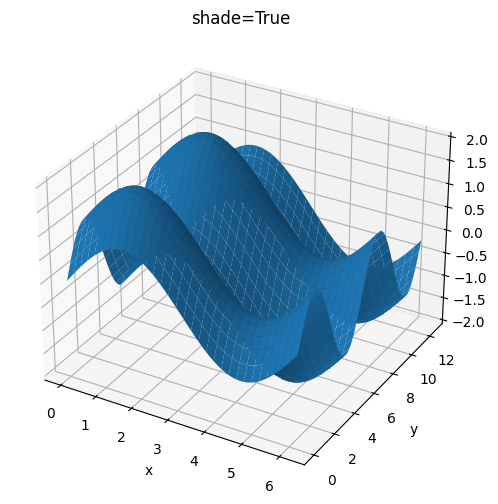
シェーディング（陰影）

ax.plot_surface()メソッドのshadeオプションでシェーディング（陰影）処理を行うか指定できます。True（デフォルト）の場合はシェーディング処理を行います。なお、cmapオプションでカラーマップを指定した場合、shade=Falseとなります。

fig, ax = plt.subplots(figsize=(6, 6), subplot_kw={'projection': '3d'})
ax.plot_surface(X, Y, Z, shade=True)
ax.set_xlabel("x")
ax.set_ylabel("y")
ax.set_zlabel("z")
ax.set_title("shade=True")
plt.show()

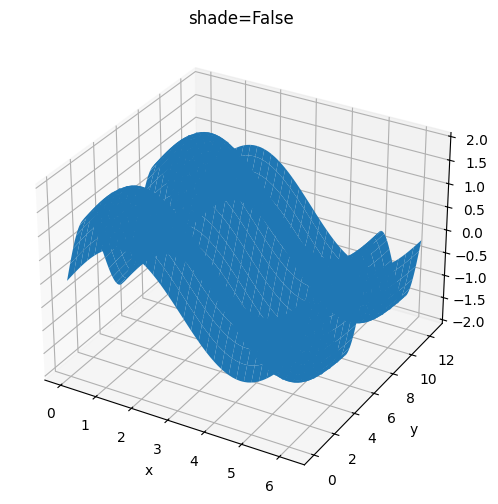
fig, ax = plt.subplots(figsize=(6, 6), subplot_kw={'projection': '3d'})
ax.plot_surface(X, Y, Z, shade=False)
ax.set_xlabel("x")
ax.set_ylabel("y")
ax.set_zlabel("z")
ax.set_title("shade=False")
plt.show()