Matplotlibのヒストグラム#
※記事内に商品プロモーションを含むことがあります。
公開日
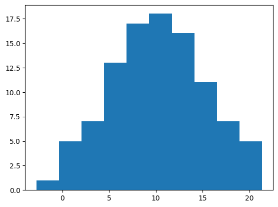
Matplotlibでヒストグラムを出力するには、ax.histを使用します。ax.histの最初の引数に表示するデータを配列で与えます。
import numpy as np
import matplotlib.pyplot as plt

np.random.seed(seed=0)
x = np.random.normal(10, 5, 100) # 平均10, 標準偏差5の正規分布で100点のデータを生成

fig, ax = plt.subplots()
ax.hist(x)
plt.show()
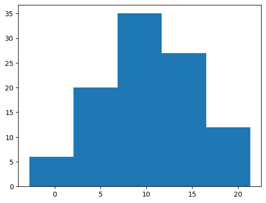
表示する棒の数はbinsオプションで指定できます(デフォルトは10)。
fig, ax = plt.subplots()
ax.hist(x, bins=5)
plt.show()
棒の太さ・色を変更する#
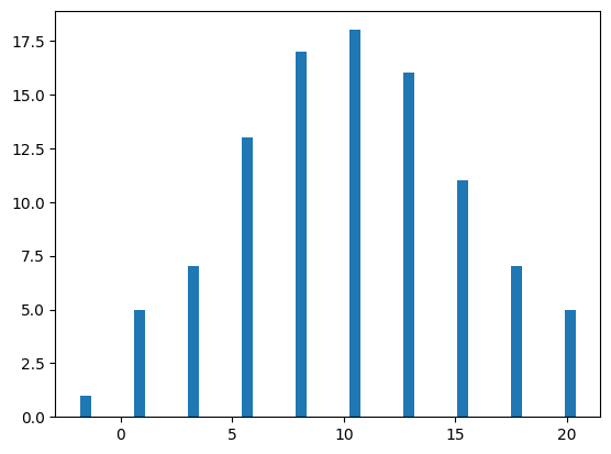
棒の太さはrwidthオプションで指定できます。0から1の範囲を取り、値が小さいほど細くなります。
fig, ax = plt.subplots()
ax.hist(x, rwidth=0.2)
plt.show()
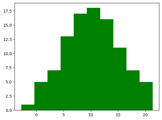
棒の色はcolorオプションで指定できます。colorオプションの詳細は以下の記事を参考にして下さい。
fig, ax = plt.subplots()
ax.hist(x, color="green")
plt.show()
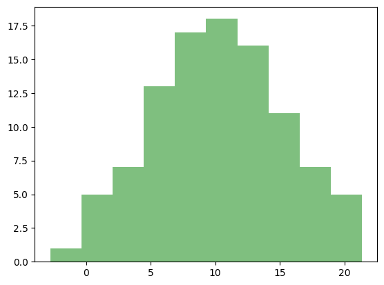
また、alphaオプションで透明度を変更できます。0から1の範囲を取り、値が小さいほど透明に近づきます。
fig, ax = plt.subplots()
ax.hist(x, color="green", alpha=0.5)
plt.show()
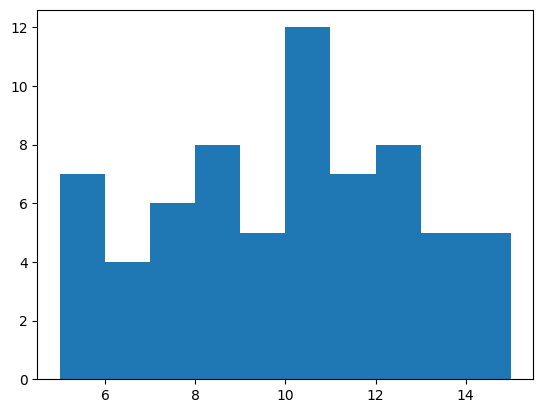
表示範囲#
表示範囲はrangeオプションで指定できます。最小値と最大値の順にタプルで与えます。rangeの外側にあるデータは無視されます。
fig, ax = plt.subplots()
ax.hist(x, range=(5, 15))
plt.show()
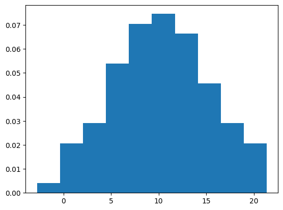
正規化#
densityオプションをTrueにすると、合計面積(棒の横幅×縦の長さの合計)が1になるように正規化されます。
fig, ax = plt.subplots()
ax.hist(x, density=True)
plt.show()
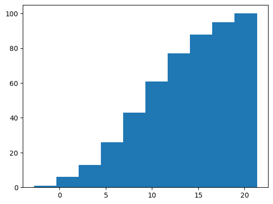
累積値#
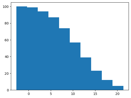
ヒストグラムを小さい値からの累積値で表示する場合、cumulativeオプションをTrueに指定します。反対に、大きい値からの累積値で表示する場合、cumulativeを-1に指定します。
fig, ax = plt.subplots()
ax.hist(x, cumulative=True)
plt.show()
fig, ax = plt.subplots()
ax.hist(x, cumulative=-1)
plt.show()
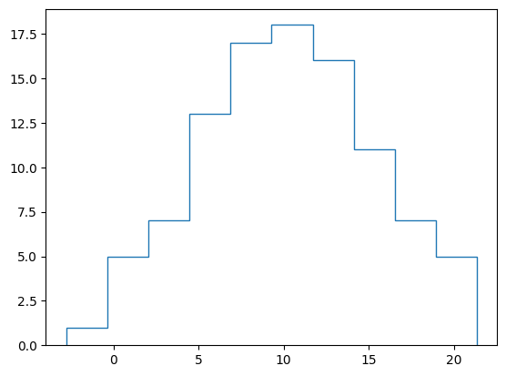
線のみのヒストグラム#
histtypeオプションを"step"にすることで、塗り潰しをしない線のみのヒストグラムになります。
fig, ax = plt.subplots()
ax.hist(x, histtype="step")
plt.show()
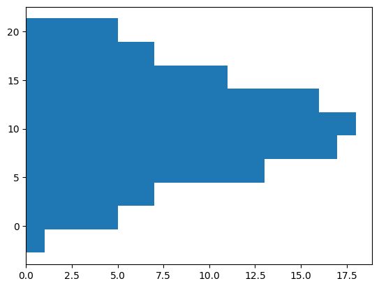
横向きのヒストグラム#
orientationオプションをTrueにすることで、ヒストグラムが横向きになります。
fig, ax = plt.subplots()
ax.hist(x, orientation="horizontal")
plt.show()
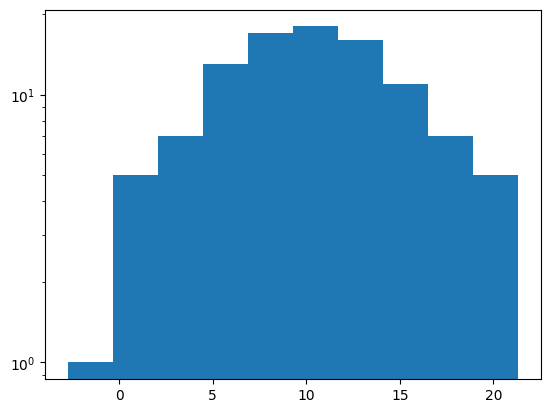
縦軸を対数にする#
logオプションをTrueとすることで、縦軸を対数表示できます。
fig, ax = plt.subplots()
ax.hist(x, log=True)
plt.show()
複数系列のヒストグラム#
複数系列のデータからヒストグラムを作成する方法を示します。
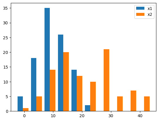
横に並べる#
まず、単純に棒を横に並べる例です。ax.histに複数のデータをリストで渡します。
np.random.seed(seed=0)
x1 = np.random.normal(10, 5, 100) # 平均10, 標準偏差5の正規分布で100点のデータを生成
x2 = np.random.normal(20, 10, 100) # 平均20, 標準偏差10の正規分布で100点のデータを生成

fig, ax = plt.subplots()
ax.hist([x1, x2])
ax.legend(["x1", "x2"])
plt.show()
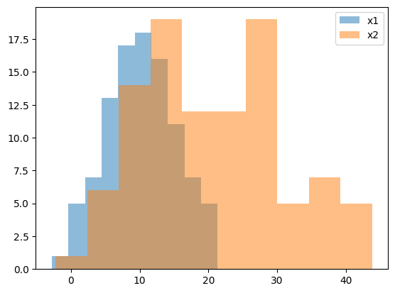
透過させて重ねる#
alphaオプションを使って棒を透過させ、重ねて表示することも可能です。
fig, ax = plt.subplots()
ax.hist(x1, alpha=0.5, label="x1")
ax.hist(x2, alpha=0.5, label="x2")
ax.legend()
plt.show()
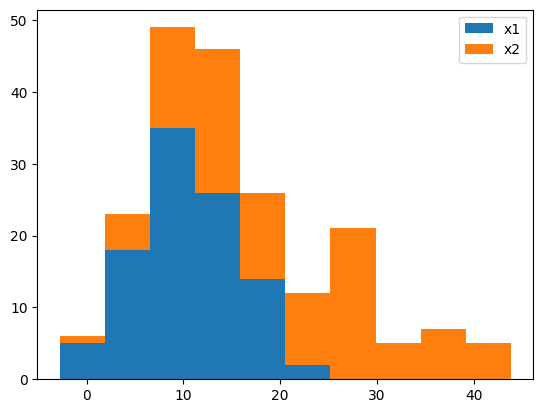
積み上げる#
ヒストグラムを積み上げる場合、histtype="barstacked"とするか、stacked=Trueとします。
fig, ax = plt.subplots()
ax.hist([x1, x2], histtype="barstacked")
# ax.hist([x1, x2], stacked=True) # これも同じ結果になる
ax.legend(["x1", "x2"])
plt.show()